8. Supplemental Sampling, Rating Curves, Loads

Last updated on 2022-12-02

Print this page

To further understand and explain the ecology of a site and lend insight into EnviroDIY Monitoring Station data patterns, a variety of additional measurements and sample collection methods can be employed. Handheld sensors, dilution kits, and other point-in-time sampling methods, as well as grab samples for laboratory analysis, can be used to gather additional explanatory information. Site specific monitoring questions will dictate which parameters are most important to investigate.

Furthermore, understanding landscape conditions in a watershed including factors such as point sources, commercial, industrial and agricultural land uses, wastewater treatment plants, and other potential sources of pollution can help in understanding and explaining EnviroDIY Monitoring Station data patterns (see WikiWatershed for a toolkit of resources to investigate these types of landscape-level data).

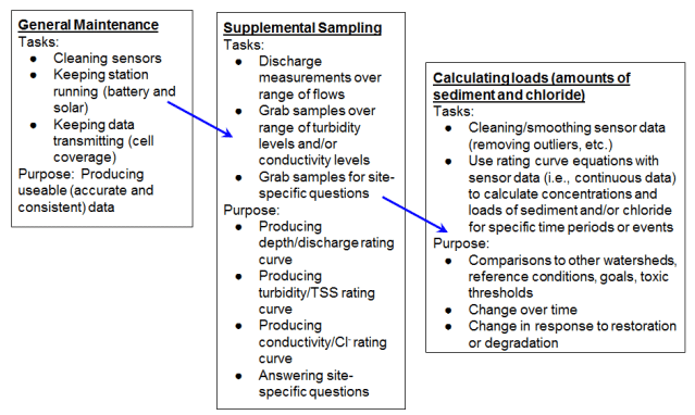
Described here is a process for collecting data that can be used to enhance the value of time series data. The supplemental sampling that is described is required when monitoring intentions dictate additional data are needed for monitoring of discharge patterns and concentrations and amounts (loads) of total suspended solids (TSS) and chloride (Cl^–). Specifically, this supplemental sampling focuses on:

• Performing discharge measurements at a range of water levels (i.e., storm flows).
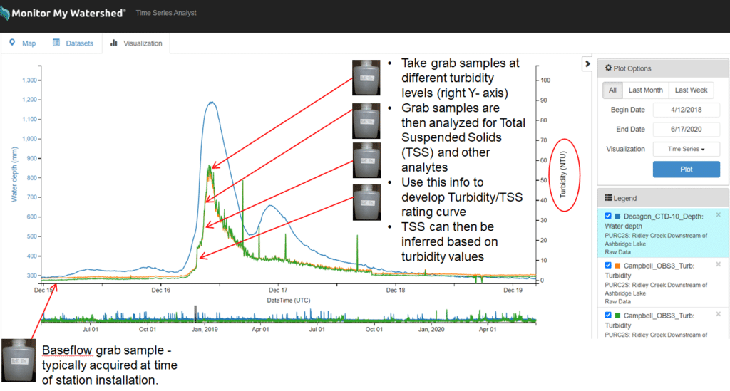
• Collecting samples of water (“grab samples”) across the range of turbidity levels observed at a site.
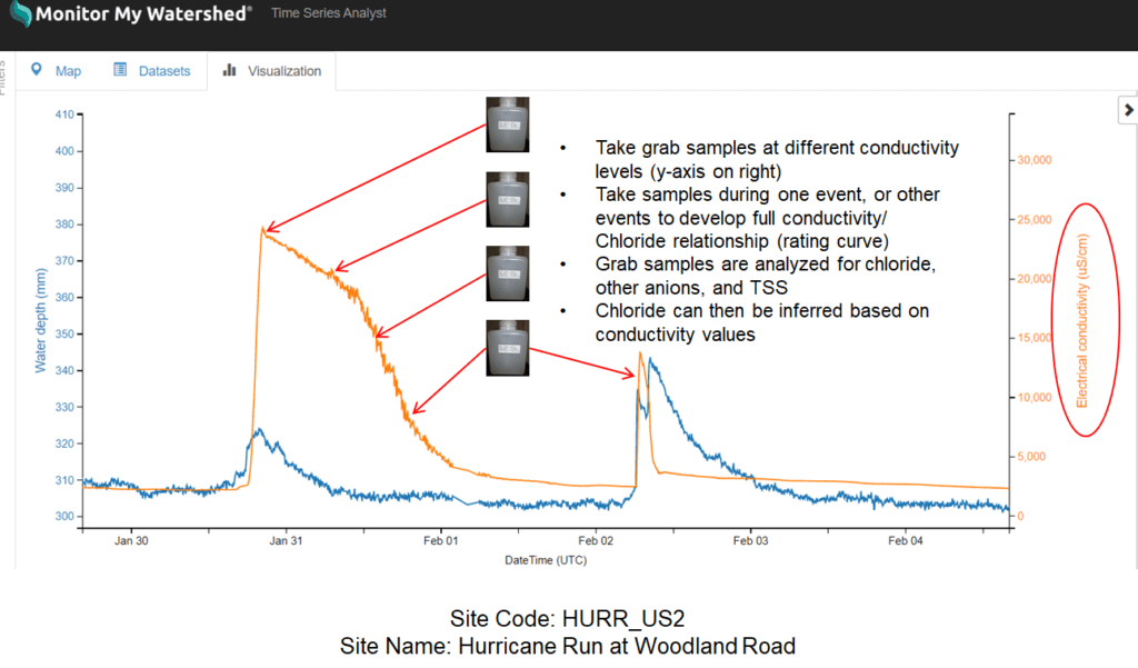
• Collecting grab samples across the range of conductivity levels observed at a site.

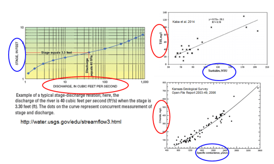
These discharge measurements and grab samples are used to develop rating curves (Figure 8.2) that describe the following relationships:

1. Sensor depth (mm) to measured discharge (m³/s)
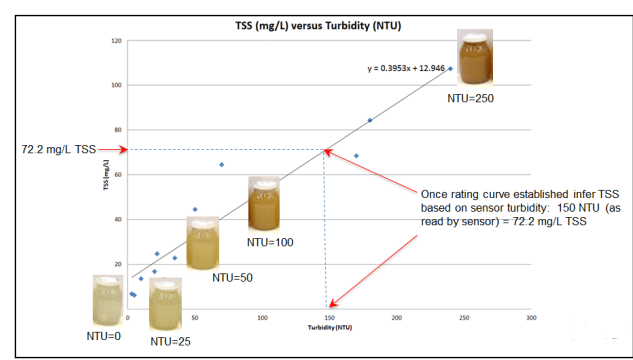
2. Sensor turbidity (NTU) to laboratory TSS (mg/L)
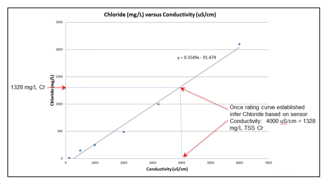
3. Sensor conductivity (μS/cm) to laboratory Cl^– (mg/L)

Once developed, regression equations from these rating curves allow the time-series monitoring station depth, turbidity, and conductivity data to be transformed to the more quantitative and ecologically informative estimates of stream discharge (m³/s), total suspended solids (TSS)(mg/L), and chloride (mg/L), respectively (see Load Calculator spreadsheet).

It is imperative that the sensors are producing accurate data when grab samples and discharge measurements are collected, so that sensor data can be matched up with the supplemental data for developing the rating curves. This means that sensors should be cleaned prior to collecting grab samples.

In high water (when grab samples are often collected) an extension for the sensor brush may be needed so that sensors can be reached for cleaning. Once discharge, TSS, and chloride data are generated via application of rating curve equations, these data can then be used to calculate amounts of water (discharge) and material (TSS load and Chloride load) moving in a stream over time (e.g., stormflow flashiness, sediment and chloride loads, identifying criteria exceedances).

The following list describes key elements of supplemental sampling and data processing associated with EnviroDIY Monitoring Stations:

• Supplemental sampling consists of:
  • Discharge measurements over a wide range of discharge to develop hydrologic rating curve.
  • Grab samples over a wide range of turbidity to develop TSS versus turbidity rating curve.
  • Grab samples over a wide range of conductivity.
  • Grab samples for answering site-specific questions.
• Supplemental sampling allows development of rating curves for depth versus discharge, TSS versus turbidity, and Cl^– versus conductivity
• Once developed, a rating curve will allow you to:
  • Infer stream discharge (m³/s) based on depth data
  • Infer Total Suspended Sediment (TSS, mg/L) concentrations based on turbidity data
  • Infer Chloride (Cl^–, mg/L) based on conductivity data
• Once you can infer this information you essentially have continuous discharge, TSS, and Chloride data, meaning you can then calculate amounts of material moving in the stream for specific time periods (i.e., loads), e.g.:
  • “During this storm event discharge quadrupled in half an hour.”
  • “During this storm event there was # kg of sediment transported by the stream.”
  • “During this snow melt event # kg of road salt (Cl^–) entered the stream.”
  • “During this salt flush event anything living in the stream was exposed to # mg/L chloride for # hours”.

8.1 Rating Curves

Instructions for developing the following three rating curves are presented here. These rating curves can then be used together and with the continuous data to calculate quantities of water, sediment (loads), and chloride (loads) moving in the stream over specific periods of time.

1. A discharge rating curve that relates sensor depth (mm, measured by CTD sensor) to discharge (m³/s; Figure 10.3).
2. A TSS versus turbidity rating curve (Figure 8.1.2.2).
3. A Cl^– versus conductivity rating curve (Figure 8.1.2.3).

See the Measuring and Predicting Discharge and Chloride, and/or Sediment Loads section of the EnviroDIY videos page to view instructional videos describing building a rating curve, discharge rating curve calculator, and stage to area predictor.

8.1.1 Discharge Rating Curve: Measuring Discharge

A Stream Discharge Data Form should be completed every time a distinct set of discharge measurements are made (see Supplemental Sampling, Rating Curves, Loads and Appendix G for details on measuring discharge). These data should then be entered and saved into the Discharge Rating Curve Calculator for that site (see Supplemental Sampling, Rating Curves, Loads).

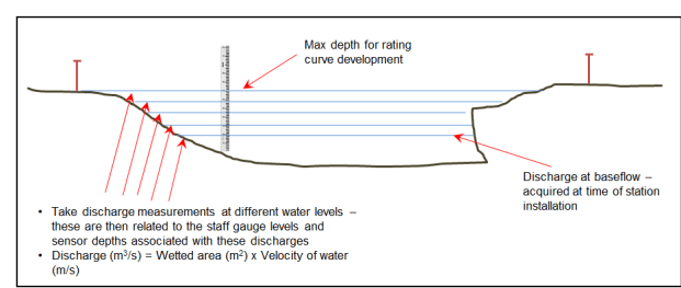
Discharge (Q, m³/s) is calculated as flow velocity (V, m/s) multiplied by wetted cross-sectional area (distance x depth = Area, m²): Q = V x A. In wadeable conditions, measurements of flow velocity and wetted area are collected using a flow meter or timed neutrally buoyant object float (velocity), meter tape (distance), and survey rod (depth). Detailed descriptions of these methods are in Appendix G.

Discharge data should be recorded on the Stream Discharge Data Form, field notebook, or other data form, and entered into the Discharge Rating Curve Calculator spreadsheet to calculate final discharge (Appendix H). These discharge data are matched with sensor depth data (same date and time) to develop the discharge rating curve.

In unwadeable conditions full cross-channel discharge measurements and wetted cross-sectional area measurements are not possible without expensive equipment. In these cases cross section wetted area can be estimated by mapping the shape/dimensions of the confined stream channel at baseflow and then using this information along with staff gauge and/or sensor depth measurements to predict cross section wetted area during unwadeable flow conditions. A method for delineating the channel cross section profile is provided in Appendix G.

Once the channel cross section has been delineated, the staff gauge water level or sensor depth can be entered into the Stage To Area Predictor spreadsheet to generate a Predicted Wetted Cross-Section Area (Appendix G). This Predicted Wetted Cross-Section Area can then be entered into the Discharge Rating Curve Calculator spreadsheet (Appendix G “Predicting Discharge” and Appendix H) with an estimate of velocity (measured with a neutral buoyant float or velocity meter) to estimate discharge.

8.1.2 Discharge Rating Curve: Generating the Discharge Rating Curve

Final discharge along with sensor depth (at the time discharge was measured) can then be incorporated into a site-specific hydrologic rating curve using the Discharge Rating Curve Calculator (e.g., Figure 8.1.2.1; see Appendix H and Instructions in the Discharge Rating Curve Calculator itself for detailed instructions).

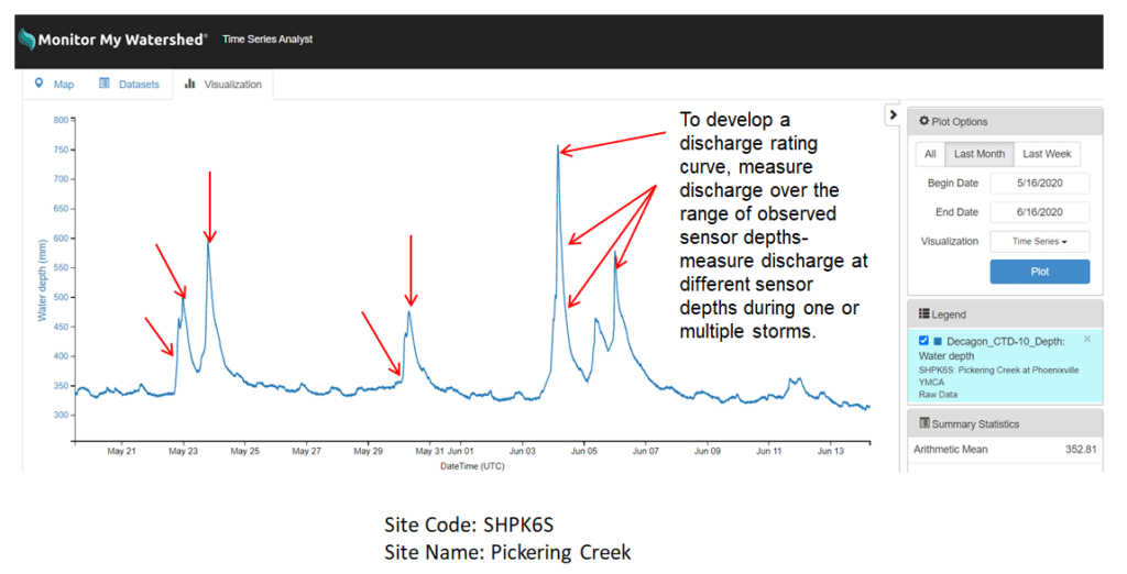
To develop a preliminary hydrologic rating curve it is recommended that at least five discharge measurements be made during stream conditions ranging from baseflow to the extreme stormflow.

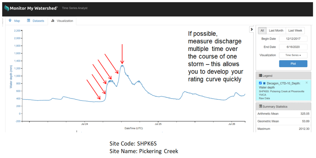
Multiple measurements can be taken during a single storm as flow rises and falls. However, it will be necessary to measure discharge in multiple storms as measuring the full range of flows within the confined channel is usually not possible during a single storm. There is no defined endpoint for when a rating curve is complete although statistical measures of the correlation coefficient and significance value can be used as a guide.

Because timing of these measurements is crucial (i.e., measurements need to be taken across a range of high flow conditions, which are often short-lived) the real-time sensor data should be used along with weather predictions and other tools (e.g., nearby USGS gauge data, first-hand knowledge) to plan for visits to conduct discharge measurements.

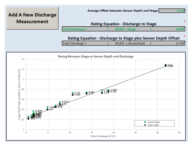
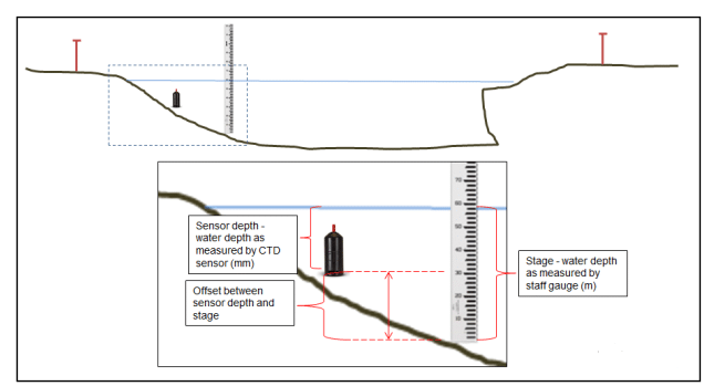
To develop the discharge rating curve it is necessary to measure discharge near the monitoring station over a range of flows (i.e., from baseflow to stormflow; Figures 8.1.2.2 and 8.1.2.3). Each time discharge is measured at a site, data should be recorded on the Stream Discharge Data Form or in a field notebook. Staff gauge height and sensor depth at the start and at the end of when measurements were taken should always be recorded. Staff gauge depth is considered the master reference and sensor depth is then related to this (sensor offset, Figure 8.1.2.4).

Discharge measurements (flow velocity, distance, and water depth), as well as staff gauge level, sensor depth and other descriptive information for the Stream Discharge Data Form are then entered into the Discharge Rating Curve Calculator, where these data are automatically incorporated into a rating curve. The equation that represents the relationship of sensor depth to discharge (i.e., the finished rating curve) can then be used along with continuous data to calculate loads using the Load Calculator spreadsheet (Appendix G).

See Appendices H and I for instructions on using the Discharge Rating Curve Calculator and Load Calculator, respectively.

8.2 Collecting Grab Samples for Rating Curves

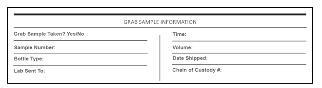
When applicable, each individual grab sample (see Supplemental Sampling, Rating Curves, Loads) collected should be documented in the Grab Sample Information section of the Field Visit Data Form on page 2. Depending on the context of the project, grab samples may be processed internally or shipped to an external lab (see Supplemental Sampling, Rating Curves, Loads).

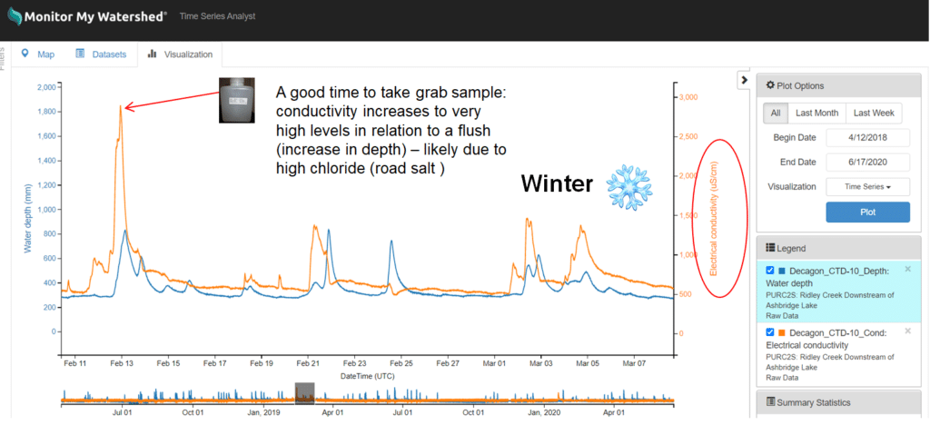
A “grab sample” is a quantity of water generally collected in a field-safe plastic bottle that is then analyzed in a lab for any number of parameters. Grab samples can be collected for any number of situational monitoring intentions. For purposes of TSS versus turbidity and Cl versus conductivity rating curve development, grab samples should be collected across the range of observed turbidity and conductivity values. For TSS versus turbidity this will mean collecting samples from during storms and low flow periods. For conductivity/Cl this will mean collecting samples when conductivity increases due to snow melt and/or rain events that carry salt into a stream, i.e., grab sample collection is timed to coincide with higher than normal conductivity levels.

Grab samples can then be processed by any number of labs for TSS and Cl, as well as many other parameters. Lab certifications, sample processing time, etc. should be assessed prior to hiring a lab to perform the required analyses to ensure resulting data are of the desired level of accuracy and precision. Examples of grab sample materials and shipping protocols are provided in Appendix L.

The basic process for collecting and shipping grab samples is:

1. Clean the sensors. It is imperative that the sensors are producing accurate data when grab samples are collected, so that sensor data can be matched up with the grab sample data for developing the rating curves. In high water (when grab samples are often collected) an extension for the sensor brush may be needed so that sensors can be reached for cleaning.
2. Collect grab sample (see below).
3. Complete grab sample, label with date and time. Make sure that time represents exact time when sample was collected.
4. Complete the Field Visit Data Form. Make sure to complete the Grab Sample Information section on the back side of the data form.
5. Make sure that date and time are exactly the same as listed on the grab sample label.
6. Place sample on ice/ice-pack or in refrigerator.
7. Prepare sample for shipping/delivery.
8. Complete any lab-required chain-of-custody forms.
9. Chill and package sample(s) according to lab protocols.
10. Ship or deliver sample to lab.
11. Note that some labs do not accept shipments on weekends. Sample collection and/or shipping should be adjusted accordingly.

Steps may vary depending on the analyte and the lab but the basic process for collecting a grab sample to be analyzed for TSS and Chloride is as follows:

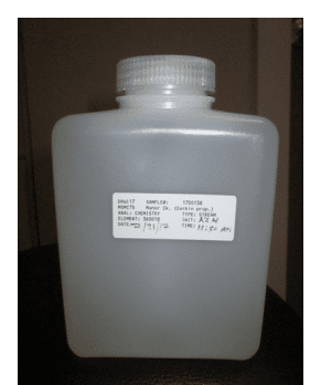
1. Rinse grab sample bottle (Figure 8.2.1) three times with typical stream water before collecting sample.
2. Fill bottle with water that is characteristic of current conditions (i.e., make sure it is from the main flow and that it does not contain material churned up from people walking in the stream).
3. Facing into the current, invert the bottle and submerge it to ⅔ total depth of the water (i.e., mouth of bottle should be facing down and bottle should not fill as you submerge it).
4. Turn the bottle right side up and begin raising the bottle through the water column at an even pace so that when the bottle reaches the surface it is filled.
5. Cap the bottle making sure that the cap is clean (rinse it with stream water if need be).
6. Fill in any header information on the grab sample label (e.g., site ID, stream name, date, and time).
7. Complete the grab sample bottle label with “Date” and “Time.” Record exact date/time (to the minute) that grab sample bottle was filled with water. This information is key when grab sample data are being used for rating curve development; the exact time is necessary so that sample data can be matched to the exact monitoring station readings from the same time.
8. Place sample immediately on ice (or ice pack) in a cooler until shipping.
9. If the Field Visit Data Form is being used, complete the Grab Sample Information section on the back side of this form, Figure 8.2.2). Make sure that date and time are the same as on the grab sample bottle label.

8.3 Generating the TSS and Chloride Rating Curves

In the context here grab sample data are used for developing rating curves for TSS versus turbidity and Cl versus conductivity (Figures 8.3.1 and 8.3.2). As with the hydrologic rating curve it is recommended that at least five samples be collected to develop each of the rating curves; however, additional samples will likely be necessary to fully articulate the rating curves.

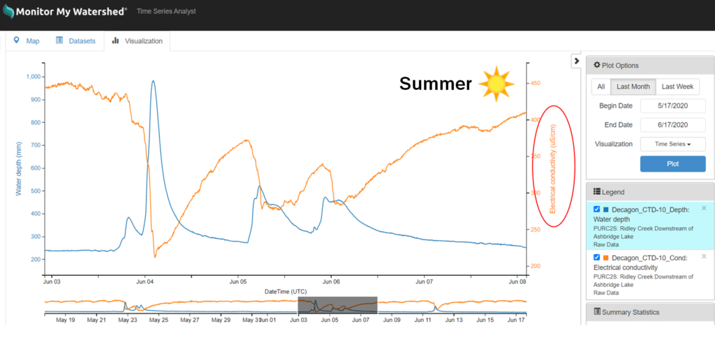
Depending on the intention for the EnviroDIY Monitoring Station data, it may make sense to develop both the TSS versus turbidity and the chloride versus conductivity curves or just one of them (e.g., if road salt input is not an issue, developing the chloride/conductivity curve would not make sense). Turbidity and conductivity ranges will be specific to the stream, so an understanding of these ranges should be established prior to collecting the grab samples. Using historic EnviroDIY Monitoring Station data, the high and low points can be identified for focusing grab sample efforts across the range.

As with the hydrologic rating curve, the grab samples can be collected from a single storm or more likely from multiple storms but, as mentioned, should be collected from across the range of observed low to high turbidity and conductivity values (Figures 8.3.3 and 8.3.4). For developing the Cl^– versus conductivity rating curve, samples will likely need to be taken during winter time salt flushes from rain or snow melt events (Figure 8.3.5). These values are then plotted against sensor data at the time grab samples were collected and the linear regression equation is generated (Figures 8.2.2 and 8.3.1) for use in final calculation of material loads.

To develop the final rating curve for TSS/turbidity or chloride/conductivity grab sample data should be graphed in a 1:1 scatterplot (e.g., Figures 8.3.1 and 8.3.2). To do this:

1. Acquire grab sample lab analysis data.
2. Match grab sample data points up with sensor data points by choosing sensor data points that are closest in time (exact minute) to when each grab sample was collected (exact minute).
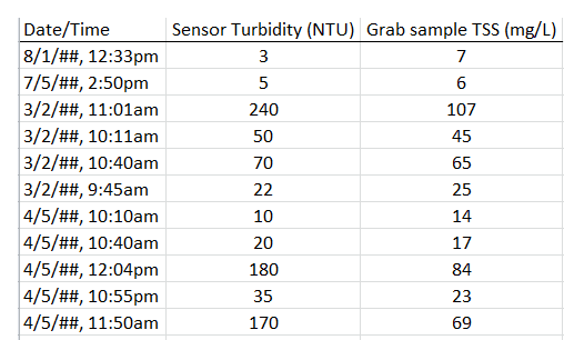
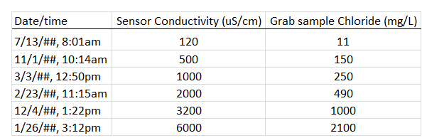
3. Add grab sample and sensor data points to Excel spreadsheet; sensor data in one column, grab sample data in another column (Tables 8.3.1 and 8.3.2)
4. Plot the data in a scatterplot, fit a linear regression line to the scatterplot, and display regression equation (Figures 8.3.1 and 8.3.2).
5. Use this equation along with the continuous sensor data in the Load Calculator spreadsheet.

8.4 Calculating Loads

Once a rating curve is developed, the equations describing the relationships between sensor depth and discharge, turbidity and TSS, and/or conductivity and chloride should be entered into the Load Calculator spreadsheet. The continuous sensor data for the time period of investigation (e.g., a single storm, a season, etc.) should also be imported into the Load Calculator. Once the rating curve equations and continuous sensor data (from a specific time range) are entered, the Load Calculator will automatically apply the rating curve equations to the sensor data and generate continuous data for the parameter that is not being directly monitored by the EnviroDIY Monitoring Station (i.e., discharge, TSS, and chloride). Once estimated continuous discharge, TSS, and/or chloride data are generated, the Load Calculator will automatically calculate fluxes of the material moving in the stream over time and sum these amounts to arrive at final loads.

See the Measuring and Predicting Discharge and Chloride, and/or Sediment Loads section on the EnviroDIY videos page for video tutorials describing how to use the Load Calculator.